Option Pricing: Overview, Components, Factors, 4 Pricing Models
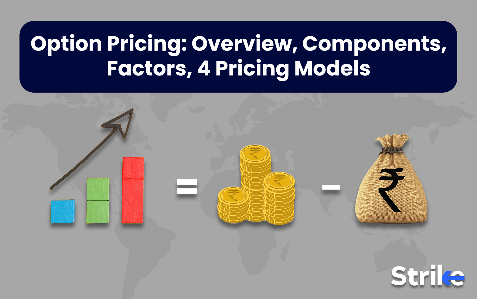


Option pricing is a pivotal aspect of options trading. Option pricing enables traders and investors to determine the fair value of an options contract. The price of an option is influenced by several factors: underlying security’s price, time-to-expiration, volatility, interest rates and more.
Options pricing is based on intrinsic and extrinsic value, determining the option contract’s profitability and time potential. Traders use options pricing models like Black-Scholes, Binomial, Monte-Carlo, and Bjerksund-Stensland Option Pricing Models to calculate the fair value of options contracts under varying market conditions.
These options pricing models account for factors such as asset price changes, market volatility, and time to expiration. Understanding these models helps traders make precise decisions, manage risks effectively, and plan strategies aligned with market trends.
What is Option Pricing?
Option pricing refers to the premium or cost you pay to buy an option contract. The pricing reflects the potential returns from the option contract. The option’s premium and profitability primarily depend on the moneyness in the contract.
Here is the table detailing the profitability in different scenarios
| Moneyness | Put Option | Call Option |
| In-the-money | The asset price is smaller than the strike price | The asset price is greater than the strike price |
| At-the-money | The strike price and security price are both equal. | The strike price and security price are both equal. |
| Out-of-the-money | The asset price is greater than the strike price. | The asset price is smaller than the strike price. |
What are the Components of Option Pricing?
The price of an option is primarily determined by the following factors:
Intrinsic Value
Intrinsic value refers to the amount you can receive if you exercise your option right now on the spot. You can find the intrinsic value by deducting the strike price from the underlying security’s current market price.
For example, suppose you own a call option with a strike price of ₹900, and the current market price of the underlying stock on the exchange is ₹1,200; the intrinsic value of the single underlying asset within the contract will be ₹300. Simply put, intrinsic value represents the profit you can gain as a contract buyer by exercising the option immediately.
Extrinsic Value
Extrinsic value, or time value, represents the segment of an option’s total price higher than its intrinsic value. This aspect is shaped by the time left until the option expires and the underlying asset’s market volatility.
For example, when an option has an intrinsic value of ₹300 and trades at ₹350, its extrinsic value amounts to ₹50. This additional value indicates the potential for the option to become more profitable before it expires.
Demand and Supply
Demand and supply are other key parameters. When demand for an option rises while supply stays constant, the price of that option increases. Conversely, when the supply of options exceeds demand, prices often fall. For instance, when many traders are interested in acquiring a particular call option, its price will increase due to a higher demand.
Which Factors Affect Option Pricing?
The following six factors influence the option pricing:
1. Underlying Asset Price
The worth of an asset under the option contract estimates an option’s worth. For example, the value of your call option contract will increase if you hold a call option on XYZ Company’s stock, and the market value of that stock rises. On the other hand, there will be a reduction in the call option’s worth if XYZ’s stock price decreases. The correlation results from the option’s intrinsic value, defined as the disparity between the asset’s market price and strike price.
2. Strike Price
A call option is more valuable when its strike price is lower than the current stock price, allowing you to buy the stock at a more favourable rate. Conversely, for put options, a higher strike price increases the option’s value because it will enable you to sell the concerned stock at a higher price.
3. Time to Expiration
The time until expiration affects option pricing due to the concept of time value. The closer an option gets to its expiration date, the more its time value erodes, known as time decay. Thus, options with longer expiration dates often carry higher premiums, allowing more time for favourable price movements in the underlying asset.
For example, consider a call option on an XYZ stock priced at ₹100 with a strike price of ₹110. Suppose the option expiry is six months away, and the premium of the ₹110 option may cost ₹500 because of the further expiry. Whereas, when expiration is within a month, the premium may lower to ₹300 or less depending upon the market condition, showing a limited period for the stock to achieve the strike price.
4. Volatility
Higher volatility means a greater probability of significant price swings in the underlying asset, boosting the chances of an option closing in-the-money by expiration. This unpredictability leads to higher option premiums, as buyers are inclined to pay more for the opportunity of more significant potential gains.
For example, suppose you buy a call option for a stock currently priced at ₹100 with an expected volatility of 10%. The option’s premium could increase if the volatility rises to 30%.
5. Interest Rate
Interest rates (Rho) directly influence option pricing by affecting the cost of carry, representing the opportunity cost of tying up capital. For call options, higher interest rates generally increase their price, as buying the stock later (by exercising the option) becomes more appealing due to potential gains from investing that money elsewhere. Conversely, put options become less expensive since holding cash is more favourable.
6. Dividends
Dividends affect the underlying stock’s price movement. When a company announces dividends, its stock price drops by about the dividend amount on the ex-dividend date. For call options, this decline makes the option less attractive to lower its value. On the other hand, when it comes to the put options, the drop raises the contract’s value, as the lower stock price increases the appeal of selling at the higher strike price.
What are the Option Pricing Models?
An option pricing model is a mathematical formula to determine the fair value of an option. They aim to quantify the components of the options contract by factoring in market dynamics and other variables. Here are the popular pricing models:
1. Black-Scholes Option Pricing Model
The Black-Scholes options pricing model is a mathematical model used to compute the price of the European call option. It considers the underlying security’s current price and volatility, the time left until expiry, and the risk-free interest rate. This formula was formulated in 1973 by Myron Scholes and Fischer Black.
Formula:
C = S0N (d1) — Ke—rTN (d2)
Where:
- (C) is the call option price
- (S_0) is the current stock price
- (K) is the strike price
- (r) is the risk-free interest rate
- (T) is the time to expiration
- N(d) shows the cumulative distribution function of the standard normal distribution.
To compute (d1) and (d2)

Black-Scholes model operates on several assumptions:
- The underlying asset’s price follows a lognormal distribution. That means their prices may rise exponentially but will not fall below zero.
- The underlying asset’s volatility stays unmoved during the option’s life. However, this assumption is not practical in real market conditions.
- The model initially assumes that the underlying asset does not distribute dividends throughout the option’s duration. However, variations such as the Black-Scholes-Merton model include dividends in their calculations.
- The markets are efficient, and all known data is already accounted for in the prices of assets.
- It assumes no chances for arbitrage, which guarantees that the option’s pricing aligns somewhat with the underlying asset’s value.
- It functions on the belief that the risk-free interest rate is fixed and remains known throughout the option’s lifespan.
2. Binomial Option Pricing Model
This option pricing model has broad applications and can be used for various conditions, including American options. Those who are unaware can exercise American options at any time before the contract expires. The binomial model was developed in 1979 by Cox, Ross, and Rubinstein. Here’s the formula for the same:
C = [pCu + (1-p)Cd]/(1+r)
Where:
- ( C ) is the contract’s current price
- (r) is the interest rate (risk-free)
- ( p ) refers to the probability of an uptrend movement in the underlying security price.
- ( C_u ) and ( C_d ) is the option prices in the up and down states
This model relies on the following assumptions:
- The underlying asset’s price can change to one of two potential values during each period, forming a binomial tree of future price possibilities.
- The model presumes that the time until expiration is segmented into distinct intervals.
- The underlying asset makes no dividend payments during the life of the option.
- The risk-free interest rate is constant throughout the life of the option.
- There are no chances for arbitrage within the marketplace.
- The markets are efficient, and all known data is already accounted for in the prices of assets.
3. Monte Carlo Simulation Pricing Model
The Monte Carlo Simulation Pricing Model generates several random samples to simulate a system’s outcomes. In options trading, it models all potential price paths for an asset. Averaging these outcomes helps estimate the option contract’s payoff. Monte Carlo Simulation is especially suitable for path-dependent Asian options. Here’s how to compute them:
Step 1: Price Modelling
Model the underlying asset price using a Geometric Brownian Motion (GBM). The model suggests that asset prices move continuously, with a steady rate of return and constant volatility. This can be expressed mathematically as:

Here,
- (S_t) is the contract’s worth at the time (t)
- (μ) is the drift rate
- (σ) is the volatility
- (dW_t) is a Wiener process that represents the random component
Step 2: Simulating Price Paths
Next, generate multiple future price paths for the underlying security using GBM. Each path represents a potential pattern the asset price might follow from the present day until the option’s expiry date.
Step 3: Payoff Calculation
Calculate the contract payoff for each simulated price path. The computation for a European contract is as follows:

Here,
- (S_t) is the worth of the security at the expiration
- (K) is the strike price
Step 4: Discounting
Determine the time value of money by discounting each payoff to its present value using the risk-free interest rate.
Step 5: Averaging
Calculate the average of all discounted payoff values to estimate the option contract price. Here is the formula:

Here,
- (N) is the number of simulations,
- (Payoffi) is the payoff from the ( i )-th simulation
- (r) is the interest rate (risk-free)
- (T) is the time to expiration
4. Bjerksund-Stensland Option Pricing Model
The Bjerksund-Stensland Options Pricing Model estimates the price of American options. The Bjerksund-Stensland was developed in 1993 by Gunnar Stensland and Petter Bjerksund. It is a closed-form solution that does not require extensive calculations. The Bjerksund-Stensland model separates the maturity period into two intervals, each with a fixed exercise limit.
Using this model, you can determine the best time to exercise the option, especially when the underlying asset price hits a specific boundary.
A vital feature of this pricing model is its consideration of continuous, constant, and discrete dividends.
Comparison of Option Pricing Models
The choice of an option pricing model depends on the type of options, market conditions, and your trading expertise. Here is a quick comparison to help you make a decision.
Black-Scholes vs. Binomial vs. Monte Carlo
| Aspect | Black-Scholes Model | Binomial Model | Monte Carlo Simulation |
| Basic Concept | It applies a closed-form formula to evaluate European option prices, and the computation is based on stable volatility and interest rates. | It uses a discrete-time approach to price options by forming a binomial tree that shows potential future stock prices. | It uses statistical modelling and random sampling techniques to forecast the future prices of the underlying asset. |
| Mathematical Complexity | Relatively simple with a closed-form solution. | Moderately complex, involving iterative calculations. | Highly complex, requiring extensive computational power. |
| Flexibility | Limited flexibility due to its assumptions of constant volatility and interest rates. | More flexible can incorporate varying volatility and interest rates. | Highly flexible, can model a wide range of scenarios and complexities. |
| Use Cases | Best suited for pricing European options on stocks, indices, and currencies. | Suitable for pricing American options and other derivatives with early exercise features. | It is ideal for pricing exotic options and complex derivatives where other models fall short. |
Choosing the Right Model for Your Strategy
Consider the following pointers before deciding on the pricing model for your options strategy.
- Understand your contract type. If you have a European contract, you can use Black-Scholes, while the binomial model is suitable for American options contracts.
- Since different pricing models work better in varying conditions, assessing the current market scenario, including volatility and economic conditions, is crucial.
- Consider how comfortable you are with complex mathematical models. While sophisticated models may provide precise pricing, simpler models might be more user-friendly and sufficient for your trading strategy.
- Once you select a model, conduct thorough backtesting using historical data to evaluate its effectiveness. This step will help you determine if the model produces reliable results that align with your trading strategy.
How do option prices change over time?
Option prices change over time due to time decay, volatility, and fluctuations in the underlying asset price. Time decay reduces the option’s extrinsic value as the contract nears its expiry. Increased volatility increases the likelihood of gains from substantial price swings, which raises the contract prices. In contrast, changes in the underlying asset’s price directly affect the option’s intrinsic value.
Can option pricing models predict market movements?
Option pricing models compute the fair value of options by considering several factors. Although they offer valuable insights into market sentiment and implied volatility, they do not directly forecast market movements. Instead, they serve as tools for risk management and strategic decision-making.
What happens if I don’t exercise my option?
Your option expires without value, and you forfeit your right to buy or sell the underlying asset at the agreed strike price if you do not exercise your option. Brokers may exercise in-the-money options automatically on your behalf. Conversely, out-of-the-money options usually expire at zero.


Share


No Comments Yet