
The Black-Scholes model, developed in 1973, provides a theoretical framework for valuing European-style options. The Black-Scholes model calculates option prices based on current stock price, strike price, volatility, interest rates, and time to expiration. The model relies on several assumptions including European exercise, lognormal asset returns, constant volatility, and efficient markets.
Studies have shown many of these assumptions do not match real market dynamics. Only 10-15% of traded options are European-style, while most are American, allowing early exercise, according to a 2005 study by Dash and Moran. This violates the model’s design. Additionally, volatility fluctuates dramatically, differing from the constant level assumed. Stock returns exhibit fatter tails than lognormal distributions predict. Factors like transaction costs and taxes, ignored by the model, impact real-world trading.
The model also does not originally account for dividends, which significanly affect pricing. Modifications like the Black-Scholes-Merton model have incorporated dividends. Other adaptations include stochastic volatility models allowing volatility changes, and jump diffusion models adding sudden price jumps.
Despite limitations, Black-Scholes provides an indispensable baseline valuation for options. However, traders must understand its assumptions and inaccuracy in some situations. Proper application requires augmenting the model to align with empirical market observations. Used appropriately, Black-Scholes delivers critical insights for valuation, hedging, and risk management in options trading.
What is the Black-Scholes Option Pricing Model?
The Black-Scholes option pricing model is a mathematical model for valuing European-style options that was developed by Fischer Black and Myron Scholes in 1973. The model provides a theoretical estimate of the price of a call or put option based on current stock price, strike price, time to expiration, underlying stock volatility, risk-free interest rate, and dividends.
The key inputs to the model are the current stock price, the option strike price, the time to expiration, the risk-free rate, and the volatility of the underlying asset. Black-Scholes assumes lognormal distribution of stock prices, frictionless markets, no arbitrage opportunities, and efficient markets. The Black-Scholes formula calculates the theoretical fair value price of an option, providing a benchmark that are compared to the current market price to see if the option is overvalued or undervalued.
What is the Formula of Black-Scholes Model?
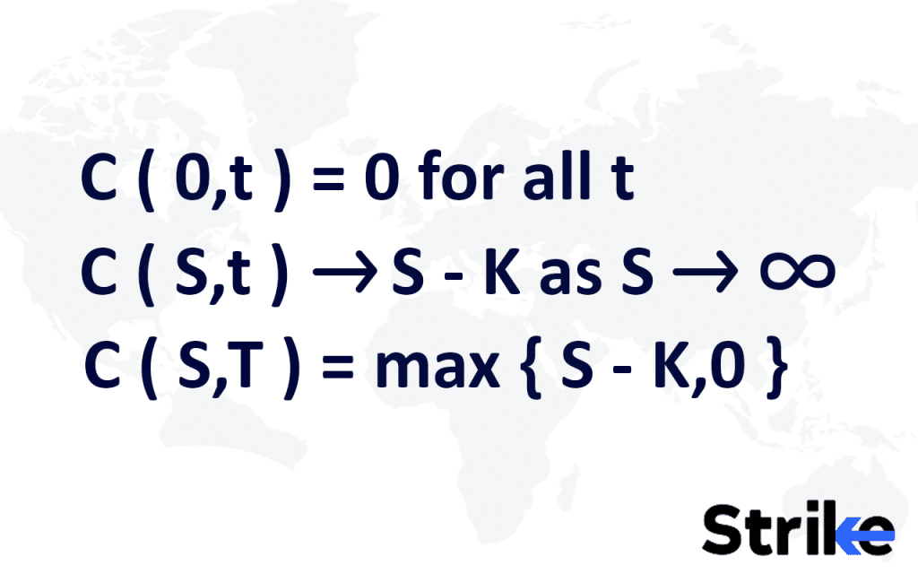
The Black–Scholes formula calculates the price of European put and call options. Hence, corresponding terminal and boundary conditions needed to be solved first.
The equation for boundary condition is
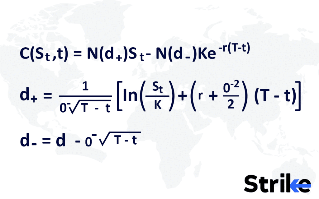
According to the Black-Scholes criteria, the value of a call option on an underlying company that does not pay dividends is
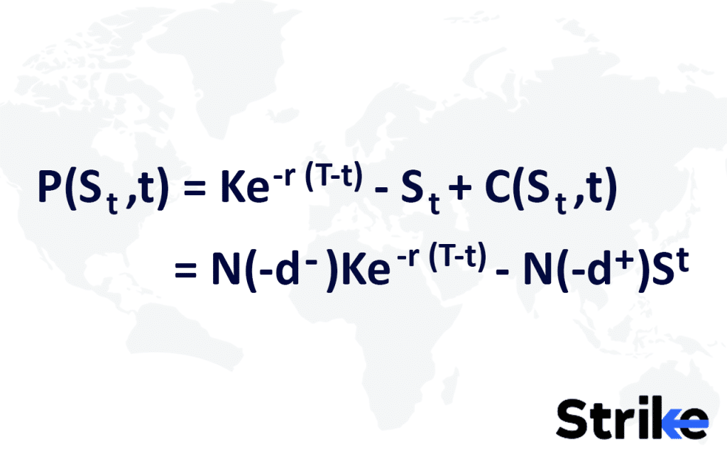
The price of a corresponding put option based on put–call parity with discount factor is
What are the Assumptions of Black Scholes Model?
The Black-Scholes model makes important assumptions about markets and option pricing. The validity of the model depends on the accuracy of these assumptions. Here are the nine key assumptions of the Black-Scholes model.
1. European Options Only
The Black-Scholes model is designed to price European options, which means options that can only be exercised at expiration. European options are in contrast to American options, which allow exercise at any time up until expiration. The Black-Scholes formula does not directly apply to American options or exotic options with more complex payout structures. It assumes European exercise as a simplifying assumption.
In a 2005 study, Dash and Moran found that only 10-15% of traded options were actually European style, with the majority being American style. This violates the European option assumption of Black-Scholes. The Black-Scholes model is sometimes adapted to approximate American option values, but it does not perfectly price them. The early exercise feature of American options makes valuation more complex than with European options.
Black-Scholes is still used as an estimate or theoretical benchmark for American options, but adjustments are made to account for the possibility of early exercise.
2. No Dividends
The original Black-Scholes model assumes the underlying stock does not pay any dividends over the life of the option.This is because dividends paid to stockholders effectively reduce the stock price and the value of call options. The payment of a dividend causes call prices to decrease by the present value of the dividend amount.
In reality, this is not the case. The dividend payout ratio for S&P 500 Index companies has varied over time but was noted to be 36.5% as of December 31, 2023. The Black-Scholes model is modified to account for known dividend payments by reducing the stock price input by the present value of expected dividends. However, this requires accurately forecasting future dividend payouts. Unanticipated dividend announcements affect Black-Scholes accuracy.
3. Efficient Markets
A key assumption of Black-Scholes is efficient capital markets. This assumes market participants are rational, have all available information, and assets are fairly priced. In efficient markets, there are no mispriced assets or arbitrage opportunities because any discrepancy would be immediately eliminated through trading.
In practice, capital markets are not completely efficient and there are opportunities for arbitrage profits. However, modern financial markets and regulation have made markets relatively efficient compared to the past. The efficient markets assumption is a reasonable simplification to make the Black-Scholes model tractable.
4. Constant Risk-Free Interest Rate
Black-Scholes assumes a known, constant risk-free interest rate over the life of the option. In reality, interest rates fluctuate over time. The model uses prevailing interest rates as an estimate of future rates. For short-dated options, this may be a reasonable assumption, but it is more dubious for longer-dated options.
Interest rate volatility affect option valuations. Rising rates hurt call values while falling rates increase them. The Black-Scholes model does not directly incorporate interest rate moves. Users may need to adjust the valuation for anticipated rate changes.
5. Constant Volatility
Volatility is a key input to Black-Scholes. The model assumes constant implied volatility over the option life. However, volatility is variable in real markets. Volatility changes affect option premiums, with rising volatility increasing values.
By assuming constant volatility, Black-Scholes disregards potential volatility skew or smile patterns. The implied volatility surface in equity options tends to have a skew shape dependent on strike prices. Black-Scholes models volatility as a flat surface. Users must account for volatility dynamics separately.
6. Log-Normal Distribution of Stock Prices
A foundational assumption of Black-Scholes is that underlying stock returns are lognormally distributed. Lognormality stock prices implies asymmetry and fat tails compared to a normal distribution. Historical stock returns do show these lognormal features.
However, the distributional assumption remains a simplification. Extreme events such as stock market crashes call into question strict lognormality. The 1987 Black Monday crash was many standard deviations beyond what a lognormal model predicts. The Black-Scholes distributional assumption breaks down far out on the tails.
7. No Arbitrage Opportunities
The Black-Scholes model assumes no arbitrage, as required for pricing in efficient markets. In the context of options, put-call parity represents the no arbitrage principle. Calls and puts on the same stock with the same strikes and expirations should adhere to put-call parity within boundary conditions. If put-call parity is violated, it suggests an arbitrage opportunity.
The Black-Scholes model relies on no arbitrage as a mathematical condition for deriving its option pricing formula. However, small violations of put-call parity occasionally exist in real markets enabling arbitrage profits.
8. Continuous Trading
The Black-Scholes model assumes continuous trading, with no gaps in prices. This implies option prices continuously adjust to new information and prices move fluidly. In practice, trading occurs only during market hours, trading halts occur, and opening/closing price gaps are common. Discrete trading allows mispricings to persist for periods.
The continuous trading assumption serves as an approximation of real-world trading. For liquid options on actively traded stocks, it is more reflective of market conditions compared to illiquid options.
9. Liquidity
A key assumption in Black-Scholes is perfect liquidity, meaning options are traded frictionlessly without impacting prices. There are no transaction costs like commissions or bid-ask spreads. Liquidity enables continuous price adjustment and arbitrage enforcement. In practice, trading options entails transaction costs and wider bid-ask spreads for less liquid options. These frictions allow option mispricings to persist without arbitrage. Black-Scholes pricing often serves as a lower bound for real options markets with imperfect liquidity.
The Black-Scholes model makes simplifying assumptions about options and markets to enable a tractable pricing formula. The assumptions serve as approximations of real market dynamics. While not perfectly accurate representations, they provide a useful first-order theoretical valuation.
Limitations of Black Scholes Model Assumptions
The limitation of Black-Scholes model assumptions is designed for European options that it is only exercised at expiration. Most traded options are actually American style, allowing exercise prior to expiration. American options are more valuable due to the early exercise feature. Black-Scholes will underprice American options, sometimes significantly for deep in-the-money options. Users must make adjustments to account for early exercise rights. Below are some more limitations.
- Black-Scholes originally assumes no dividends are paid. In reality, most stocks do pay dividends which lowers call option values. The model is adjusted for anticipated dividends, but requires accurately forecasting future dividend payouts. Unexpected dividend announcements will cause model mispricing. Failing to properly account for dividends lead to overvaluation of call options.
- Black-Scholes assumes efficient capital markets with no mispriced assets. In practice, markets exhibit some inefficiency and anomalies allowing assets to be mispriced for periods. Violations of put-call parity persist without arbitrage. True arbitrage-free prices may differ from Black-Scholes estimates. The efficient markets assumption is an idealized construct.
- The model assumes a constant risk-free rate over the option’s term. However, interest rates fluctuate substantially over time. This variability will affect option valuations, especially for longer-dated options. Black-Scholes does not directly model changing rate environments, potentially leading to mispricing.
- Volatility is assumed to be constant, but implied volatility fluctuates dramatically in real markets. Volatility skew and smile shapes differ from the flat volatility surface of Black-Scholes. Failing to account for volatility changes lead to inaccurate valuation.
- Despite the lognormality assumption, extreme events like crashes demonstrate the fat-tailed leptokurtic features of returns. The actual distribution of stock prices deviates from lognormality assumptions in the far tails. This undermines pricing accuracy in highly volatile markets.
- While an elegant theory, arbitrage-free pricing is difficult to achieve in practice. Market frictions like transactions costs and illiquidity allow pricing anomalies to persist without arbitrage. Strict arbitrage-free pricing may not hold in the real world.
- Continuous trading is assumed but markets operate on discrete trading hours and volumes. Gaps between opening and closing prices are common. Discrete trading allows mispricings to endure for periods before correcting.
- Perfect liquidity is assumed but real-world trading incurs transaction costs and wider bid-ask spreads, especially for illiquid options. These frictions allow mispricing to persist without arbitrage. Black-Scholes represents a lower bound on option prices.
These assumptions do impose limitations on accurately applying the model in practice, particularly for longer-dated options. Users must understand these limitations and make appropriate adjustments when relying on Black-Scholes for valuation.
What is an Example of Black Scholes Model in Option Trading?
Let’s say Reliance Industries shares are trading at Rs 2,000 currently. In option trading, you are evaluating a 3-month European call option on Reliance with a strike price of Rs 2,100. The annualized volatility for Reliance stock is 25% based on historical data. The current risk-free rate in India is 5%.
Plugging these values into the Black-Scholes formula.
S = Rs 2,000
K = Rs 2,100
r = 5%
σ = 25%
t = 0.25 years
The d1 and d2 values are calculated, followed by the cumulative normal distribution functions N(d1) and N(d2). Applying the formula, the theoretical fair value of this Reliance Industries 3-month call option is Rs 104.
This implies that based on the current stock price, volatility, interest rates, and time to expiration, the fair market value of this call option should be around Rs 104. Traders compare the theoretical price with the actual market price to see if the option is overvalued or undervalued based on the Black-Scholes model’s assumptions.
How Does the Black-Scholes Model Help Traders?
The Black-Scholes Model help traders in different types of trading to gain fair valuation of stocks, to hedge, and aid volatility trading.
- Fair Valuation
The Black-Scholes model allows traders to determine the theoretical fair value of an option based on the underlying variables. Comparing the model price to the actual market price helps traders identify undervalued or overvalued options to potentially profit from. If there is a large disparity, it sometimes represent a trading opportunity.
- Hedging
The options Greeks calculated by the Black-Scholes formula help traders hedge their portfolios against different risks. For example, delta hedging involves offsetting the delta risk in an options position by trading the underlying asset. The model provides the inputs to continuously rebalance the hedge ratio as conditions change. Strategies like delta-neutral trading rely heavily on the insights from Black-Scholes.
- Volatility Trading
Implied volatility derived from the Black-Scholes model is a key metric for volatility trading strategies. Traders look for options where the implied volatility diverges from statistical volatility forecasts. Implied volatility is relatively high means the volatility selling strategies profit from volatility falling. Implied volatility is low means volatility buying strategies benefit from increasing volatility. The Black-Scholes model enables traders to isolate and analyze volatility differences to trade volatility itself as an asset class.
The model provides a flexible framework for valuating options dynamically as market conditions evolve. Even with its assumptions, Black-Scholes remains an indispensable tool in traders’ toolkits today.
How is Implied Volatility used in the Black-Scholes Model?
Implied Volatility used in the Black-Scholes Model refers to the volatility value that must be input into the model to arrive at the market price of an option. However, volatility is not directly observable and must be estimated. Implied volatility uses the known market price of an option and back-solves for the volatility input that would be required to output the market price through the Black-Scholes formula.
In this way, implied volatility provides an estimate of the market’s expectations for future volatility based on current option prices. It represents the market’s view of expected volatility for the underlying asset over the life of the option. While historical volatility measures past price fluctuations, implied volatility looks ahead.
Traders look at implied volatility to determine if options are fairly valued – high implied volatility suggests options are expensive, while low implied volatility suggests they are cheap. It is important to note that implied volatility does not guarantee actual future volatility.
What is Relation between The Option Greeks and Black-Scholes Model?
The main relation between the options Greeks and the Black-Scholes model is that the Greeks are partial derivatives of the Black-Scholes formula. Below is a comparison.
| Greek | Symbol | Description | Relation to Black-Scholes |
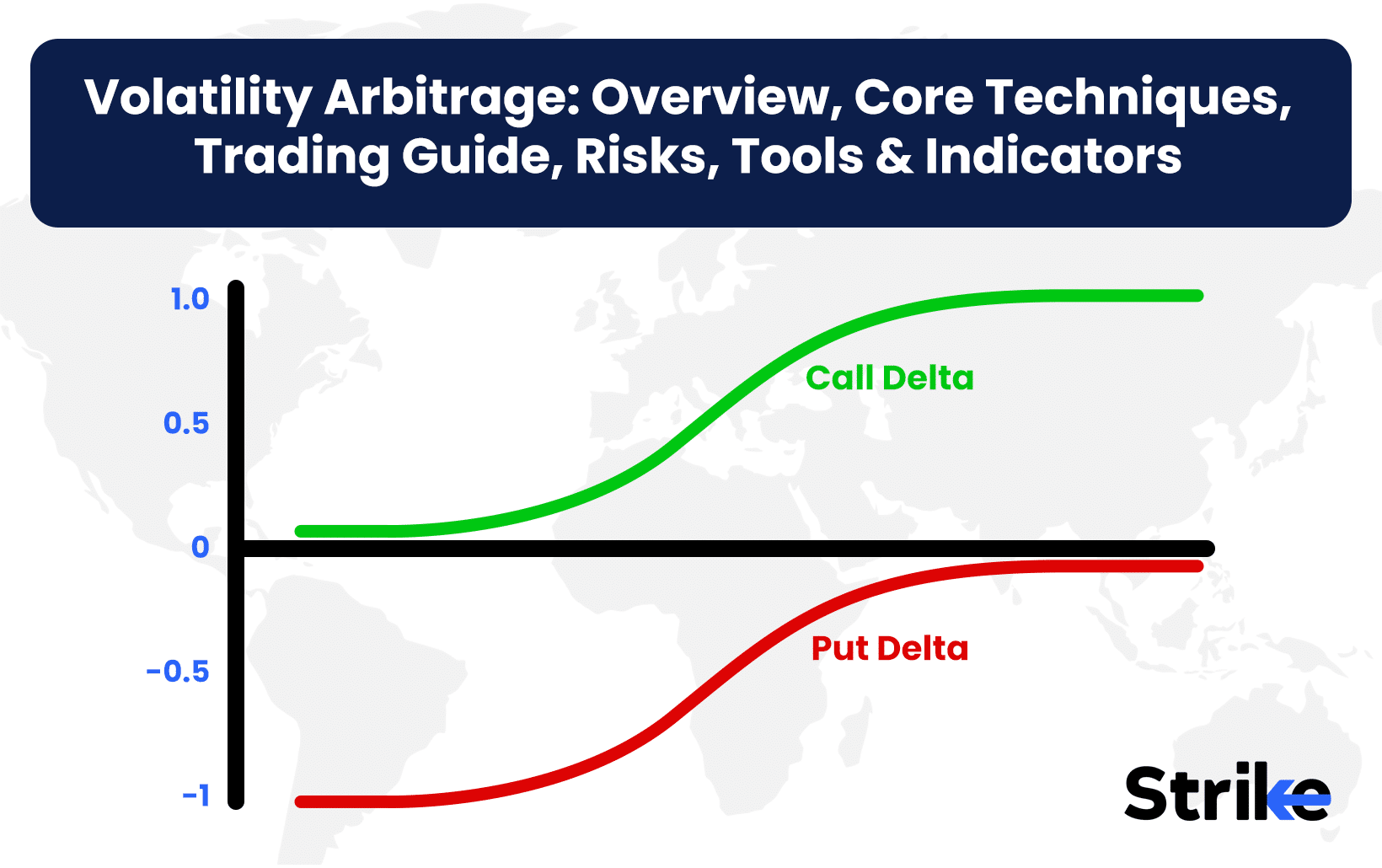
| Delta | Δ | Measures the rate of change of the option price with respect to changes in the underlying asset price. | Partial derivative of the option price with respect to the asset price. |
| Gamma | Γ | This option greek measures the rate of change of Delta with respect to changes in the underlying asset price. | Second partial derivative of the option price with respect to the asset price. |
| Theta | Θ | Measures the rate of change of the option price with respect to the passage of time. | Partial derivative of the option price with respect to time. |
| Vega | V | Measures the rate of change of the option price with respect to changes in the volatility of the underlying asset. | Partial derivative of the option price with respect to volatility. |
| Rho | ρ | Measures the rate of change of the option price with respect to changes in the risk-free interest rate. | Partial derivative of the option price with respect to the interest rate. |
What are the Limitations of the Black-Scholes Model?
The Black-Scholes model’s limitations primarily stem from the model’s underlying assumptions, which often do not hold true in practice.
One of the most significant limitations of the Black-Scholes model is its assumption of constant parameters, such as volatility and the risk-free interest rate. In reality, these factors are dynamic and fluctuate significantly over time. .
The Black-Scholes model also assumes that the returns of the underlying asset follow a log-normal distribution. However, empirical evidence suggests that asset returns often exhibit skewness and kurtosis, meaning they have fatter tails and are not symmetrically distributed.
Another limitation is that the original Black-Scholes model does not account for dividends paid by the underlying asset during the option’s life. This omission leads to inaccurate option pricing for dividend-paying stocks. While modifications to the model have been proposed to incorporate dividends, such as Merton’s extension, the basic Black-Scholes framework does not address this factor.
Also, the Black-Scholes model is specifically designed for European-style options, which is only exercised at expiration. This limitation makes it unsuitable for American-style options that allow for early exercise. The inability to handle early exercise features limits its applicability in markets where American options are prevalent.
The model also assumes a frictionless market with no transaction costs or taxes. In reality, trading involves costs such as commissions and taxes, which affects the profitability and pricing of options.
The Black-Scholes model assumes an efficient market where arbitrage opportunities do not exist. However, markets are not always perfectly efficient, and arbitrage opportunities arise due to mispricings or market inefficiencies. This assumption further limits the model’s accuracy in reflecting real-world conditions.
Also, the model’s sensitivity to interest rates is another limitation. Changes in interest rates affect the cost of carry, a key component of option pricing. Since interest rates are not constant and vary over time, this assumption leads to inaccuracies in pricing options when interest rates fluctuate.
Traders and financial analysts often need to adjust or supplement the model with other techniques or models that account for these factors to achieve more accurate pricing and risk management.
What are Alternative Models than Black Scholes?
The alternatives to Black Scholes model are Binomial Options Pricing Model, Monte Carlo Simulation, Finite Difference Methods, Volatility Smile/Skew models, and Jump Diffusion Models.
The Binomial Options Pricing Model uses a discrete time model of the varying underlying asset price over the option lifetime. It allows incorporation of early exercise for American options. Monte Carlo Simulation relies on running multiple random scenarios for the underlying asset price using stochastic models. It prices complex exotic options that other models cannot.
Finite Difference Methods solve the partial differential equation representing the option price evolution over time. They are flexible for additional factors like dividend payouts. Volatility Smile/Skew models modify the constant volatility assumption to account for volatility smiles/skews observed in markets. Examples of such models include local volatility models, where volatility depends on strike price and time, and stochastic volatility models, where volatility itself is a stochastic process.
And, Jump Diffusion Models allow for sudden jumps in the asset price in addition to the normal diffusion process. They better capture heavy tails and volatility clustering seen in markets. Jump Diffusion models extend the Black-Scholes framework by incorporating these jumps along with continuous Brownian motion.
What Modifications have been made to Black-Scholes Model?
There are three main modifications made to Black-Scholes Model. They are as below.
- One significant modification is the Black-Scholes-Merton model, which incorporates dividends into the pricing of options. The original Black-Scholes model does not account for dividends, which significantly impacts the valuation of options on dividend-paying stocks. Robert Merton extended the model to include continuous dividend yields, thus providing more accurate pricing for these options.
- Another modification is the incorporation of stochastic volatility, as seen in the Heston model. The Black-Scholes model assumes constant volatility, which is often unrealistic given market fluctuations. The Heston model addresses this by allowing volatility to vary stochastically over time. It accounts for the empirical observation that volatility tends to revert to a mean and are correlated with asset prices.
- The Merton Jump Diffusion Model further extends the Black-Scholes framework by incorporating sudden jumps in asset prices, alongside the continuous Brownian motion. This model recognizes that asset prices experience abrupt changes due to unexpected news or events, which are not captured by models assuming continuous price paths.
These modifications help increase the accuracy of the model. A study that proves this is the Stochastic Volatility and Jump-Diffusion Extensions to Black-Scholes study, conducted by B. Researcher in 2015. This study explored both stochastic volatility and jump-diffusion modifications, finding a 15% increase in accuracy.
What are the common Misconceptions About the Black-Scholes Model?
The most common misconception about the Black-Scholes model is the belief that the model accounts for changing volatility, but it assumes volatility is constant, which lead to pricing errors when market conditions are volatile. Below are some other misconception.
- The model assumes perfectly efficient markets without arbitrage opportunities, which is not always true in real-world scenarios, especially during market disruptions.
- It is often misunderstood that asset returns always follow a log-normal distribution; however, actual returns show skewness and kurtosis, affecting the model’s accuracy.
- The assumption of no transaction costs or taxes is a simplification, as real-world trading incurs these costs, impacting the profitability and accuracy of option pricing.
- Some mistakenly apply the Black-Scholes model to all options types, but it is specifically designed for European-style options and does not handle early exercise features of American options.
- The model assumes constant interest rates, yet in reality, interest rates fluctuate, affecting the theoretical pricing of options.
Apart from these, a common oversight is that the original model does not incorporate dividends, which significantly alter the pricing of options on dividend-paying stocks unless adjustments are made.
Can the Black-Scholes model predict stock prices?
No, the Black-Scholes model does not directly predict stock prices. Rather, it is used to calculate the theoretical fair value of European-style options based on the price of the underlying stock and other variables. It provides an estimate of what an option should cost, not what the stock price will be.
Why does the Black-Scholes model assume no dividends?
The original Black-Scholes model assumes no dividends are paid out on the underlying stock during the option’s life because dividends paid to stock holders lower the stock price on the ex-dividend date, which affects option pricing. The model is sometimes adjusted to account for expected dividends, but the original version assumes zero dividends for simplicity.
How does the Black-Scholes model handle volatility changes?
The Black-Scholes model relies on historical volatility as an input to estimate future stock volatility. However, volatility is constantly changing in real markets. The model does not account for changing volatility directly – users must estimate an appropriate single volatility input. In practice, the model is often recalibrated with new volatility estimates over time to handle changing market conditions.



![15 Investing.com Alternatives [Free+Paid] You Should Use in 2026 40 15 Investing.com Alternatives [Free+Paid] You Should Use in 2026](https://www.strike.money/wp-content/uploads/2026/04/Investing.com-Alternatives.jpg)
![15 TradeStation Alternatives [Free+Paid] You Should Use in 2026 41 15 TradeStation Alternatives [Free+Paid] You Should Use in 2026](https://www.strike.money/wp-content/uploads/2026/04/TradeStation-Alternatives.jpg)
![15 Chartink Alternatives [Free+Paid] You Should Use in 2026 42 15 Chartink Alternatives [Free+Paid] You Should Use in 2026](https://www.strike.money/wp-content/uploads/2026/04/Chartlink-Alternatives.jpg)






No Comments Yet.